Introduction by Example: Fibonacci Sequences

An easy example that illustrates the value of computational reuse has to do with computing recursive functions. Let's consider the Fibonacci Sequence, which provides a solution to the following mathematical puzzle:

If a pair of rabbits are put into a pen, breed such that they produce a new pair of rabbits every month, and new-born rabbits begin breeding after two months, how many rabbits are there after n months? (No rabbits ever die, and no rabbits ever leave the pen or become infertile.)

Leonardo Fibonacci

Fibonacci was a 13th-century Italian mathematician who made a number of important contributions to mathematics and is often credited as signaling the rebirth of mathematics after the fall of Western science during the Dark Ages.

The answer to this riddle is what is now known as the Fibonacci Sequence. The number of rabbit pairs at month n is equal to the number of rabbit pairs the previous month (because no rabbits ever die), plus the number of rabbit pairs two months ago (because each of those is of breeding age and thus has produced a pair of baby rabbits). Mathematically, the Fibonacci Sequence is defined by these identities:

Fib(0) = 1
Fib(1) = 1
Fib(n) = Fib(n-1) + Fib(n-2)

If you expand this for say, n = 5, you get this:

Fib(5) = Fib(4) + Fib(3)

Now you know this:

Fib(4) = Fib(3) + Fib(2)

and this:

Fib(3) = Fib(2) + Fib(1)

So you expand the preceding to this:

Fib(5) = Fib(3) + Fib(2) + Fib(2) + Fib(1)

Similarly, you get this:

Fib(2) = Fib(1) + Fib(1)

Therefore, the value of Fib(5) is derived as follows:

Fib(5) = Fib(2) + Fib(1) + Fib(1) + Fib(0) + Fib(1) + Fib(0) + Fib(1)
= Fib(1) + Fib(0) + Fib(1) + Fib(1) + Fib(0) + Fib(1) + Fib(0) + Fib(1)
= 8

Thus, if you calculate Fib(5) with the straightforward recursive function:

function Fib($n) {
  if($n == 0 || $n == 1) {
    return 1;
  }
  else {
    return Fib($n - 2) + Fib($n - 1);
  }
}

you see that you end up computing Fib(4) once but Fib(3) twice and Fib(2) tHRee times. In fact, by using mathematical techniques beyond the scope of this book, you can show that calculating Fibonacci numbers has exponential complexity (O(1.6^n)). This means that calculating F(n) takes at least 1.6^n steps. Figure 11.1 provides a glimpse into why this is a bad thing.

Figure 11.1. Comparing complexities.

Introduction by Example: Fibonacci Sequences

Complexity Calculations

When computer scientists talk about the speed of an algorithm, they often refer to its "Big O" speed, written as O(n) or O(n²) or O(2ⁿ). What do these terms mean?

When comparing algorithms, you are often concerned about how their performance changes as the data set they are acting on grows. The O() estimates are growth estimates and represent a worst-case bound on the number of "steps" that need to be taken by the algorithm on a data set that has n elements.

For example, an algorithm for finding the largest element in an array goes as follows: Start at the head of the array, and say the first element is the maximum. Compare that element to the next element in the array. If that element is larger, make it the max. This requires visiting every element in the array once, so this method takes n steps (where n is the number of elements in the array). We call this O(n), or linear time. This means that the runtime of the algorithm is directly proportional to the size of the data set.

Another example would be finding an element in an associative array. This involves finding the hash value of the key and then looking it up by that hash value. This is an O(1), or constant time, operation. This means that as the array grows, the cost of accessing a particular element does not change.

On the other side of the fence are super-linear algorithms. With these algorithms, as the data set size grows, the number of steps needed to apply the algorithm grows faster than the size of the set. Sorting algorithms are an example of this. One of the simplest (and on average slowest) sorting algorithms is bubblesort.bubblesort works as follows: Starting with the first element in the array, compare each element with its neighbor. If the elements are out of order, swap them. Repeat until the array is sorted. bubblesort works by "bubbling" an element forward until it is sorted relative to its neighbors and then applying the bubbling to the next element. The following is a simple bubblesort implementation in PHP:

[View full width]
function bubblesort(&$array) { $n = count($array); for($I = $n; $I >= 0; $I--) { // for every position in the array for($j=0; $j < $I; $j++) { // walk forward through the array to that spot if($array[$j] > $array[$j+1]) { // if elements are out of order then swap position j and j+1 list($array[$j], $array[$j+1]) = array($array[$j+1], $array[$j]); } } } }

In the worst-case scenario (that the array is reverse sorted), you must perform all possible swaps, which is (n² + n)/2. In the long term, the n² term dominates all others, so this is an O(n²) operation.

Figure 11.1 shows a graphical comparison of a few different complexities.

Anything you can do to reduce the number of operations would have great long-term benefits. The answer, though, is right under your nose: You have just seen that the problem in the manual calculation of Fib(5) is that you end up recalculating smaller Fibonacci values multiple times. Instead of recalculating the smaller values repeatedly, you should insert them into an associative array for later retrieval. Retrieval from an associative array is an O(1) operation, so you can use this technique to improve your algorithm to be linear (that is, O(n)) complexity. This is a dramatic efficiency improvement.

Note

You might have figured out that you can also reduce the complexity of the Fibonacci generator to O(n) by converting the tree recursive function (meaning that Fib(n) requires two recursive calls internally) to a tail recursive one (which has only a single recursive call and thus is linear in time). It turns out that caching with a static accumulator gives you superior performance to a noncaching tail-recursive algorithm, and the technique itself more easily expands to common Web reuse problems.

Before you start tinkering with your generation function, you should add a test to ensure that you do not break the function's functionality:

<?
require_once 'PHPUnit/Framework/TestCase.php';
require_once 'PHPUnit/Framework/TestSuite.php';
require_once 'PHPUnit/TextUI/TestRunner.php';

require_once "Fibonacci.inc";

class FibonacciTest extends PHPUnit_Framework_TestCase {
  private $known_values = array( 0 => 1,
                             1 => 1,
                             2 => 2,
                             3 => 3,
                             4 => 5,
                             5 => 8,
                             6 => 13,
                             7 => 21,
                             8 => 34,
                             9 => 55);

  public function testKnownValues() {
    foreach ($this->known_values as $n => $value) {
      $this->assertEquals($value, Fib($n),
                          "Fib($n) == ".Fib($n)." != $value");
    }
  }
  public function testBadInput() {
    $this->assertEquals(0, Fib('hello'), 'bad input');
  }
  public function testNegativeInput() {
    $this->assertEquals(0, Fib(-1));
  }
}
$suite = new PHPUnit_Framework_TestSuite(new Reflection_Class('FibonacciTest'));
PHPUnit_TextUI_TestRunner::run($suite);
?>

Now you add caching. The idea is to use a static array to store sequence values that you have calculated. Because you will add to this array every time you derive a new value, this sort of variable is known as an accumulator array. Here is the Fib() function with a static accumulator:

function Fib($n) {
  static $fibonacciValues = array( 0 => 1, 1 => 1);
  if(!is_int($n) || $n < 0) {
    return 0;
  }
  If(!$fibonacciValues[$n]) {
   $fibonacciValues[$n] = Fib($n  2) + Fib($n  1);
  }
  return $fibonacciValues[$n];
}

You can also use static class variables as accumulators. In this case, the Fib() function is moved to Fibonacci::number(), which uses the static class variable $values:

class Fibonacci {
  static $values = array( 0 => 1, 1 => 1 );
  public static function number($n) {
    if(!is_int($n) || $n < 0) {
      return 0;
    }
    if(!self::$values[$n]) {
      self::$values[$n] = self::$number[$n -2] + self::$number[$n - 1];
    }
    return self::$values[$n];
  }
}

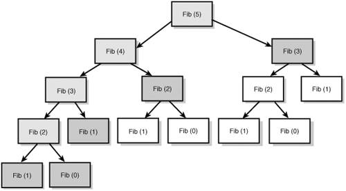
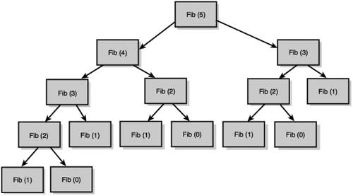
In this example, moving to a class static variable does not provide any additional functionality. Class accumulators are very useful, though, if you have more than one function that can benefit from access to the same accumulator.

Figure 11.2 illustrates the new calculation tree for Fib(5). If you view the Fibonacci calculation as a slightly misshapen triangle, you have now restricted the necessary calculations to its left edge and then directed cache reads to the nodes adjacent to the left edge. This is (n+1) + n = 2n + 1 steps, so the new calculation method is O(n). Contrast this with Figure 11.3, which shows all nodes that must be calculated in the native recursive implementation.

Figure 11.2. The number of operations necessary to compute `Fib(5)` if you cache the previously seen values.

Introduction by Example: Fibonacci Sequences

Figure 11.3. Calculations necessary for `Fib(5)` with the native implementation.

We will look at fine-grained benchmarking techniques Chapter 19, "Synthetic Benchmarks: Evaluating Code Blocks and Functions," but comparing these routines side-by-side for even medium-size n's (even just two-digit n's) is an excellent demonstration of the difference between a linear complexity function and an exponential complexity function. On my system, Fib(50) with the caching algorithm returns in subsecond time. A back-of-the-envelope calculation suggests that the noncaching tree-recursive algorithm would take seven days to compute the same thing.

Table of Contents

Introduction by Example: Fibonacci Sequences